Automatic Partition Splitting — An Epic Usability Upgrade for OceanBase

Background

As digitalization advances, the volume of business data handled by today’s databases has surged, and a single table can easily reach an enormous scale. At this point, a standalone database often cannot accommodate such large workloads, so you need the scaling capability of a distributed database to spread the data across multiple nodes and achieve load balancing.

In OceanBase, load balancing is achieved by partitioning a table and distributing the data across different cluster nodes at partition granularity. But this relies on the user being able to design reasonable partitioning rules to make good use of horizontal scaling. That not only requires a thorough understanding of the various partitioning methods, but also a deep understanding of how the business uses the database. In some scenarios, manual partitioning even makes it difficult to achieve an outcome that is optimal on all fronts.

The automatic partition splitting feature can automatically split partitions based on a user-defined partition size threshold, allowing users to make good use of OceanBase’s distributed capabilities without having to worry about partition planning.

This article first introduces the pain points of manual partitioning, then describes how automatic partitioning solves these problems, and finally covers the characteristics of automatic partitioning in detail, including its use cases, usage, and limitations.

Pain Points of Manual Partitioning

The goal of load balancing in a distributed database is to keep resource usage across nodes as balanced as possible. To achieve this, you need to design reasonable partitions so that resource consumption across partitions is moderate. Partitions that are too large can lead to load imbalance and space amplification during compaction, while partitions that are too small can produce excessive metadata and suboptimal performance. Before the automatic partition splitting feature was released, you typically had to design partitioning rules by hand, which is usually quite difficult. The following uses an abstracted business scenario to illustrate the pain points of manual partitioning.

Suppose there is a system with a table whose primary key is (Company ID, Employee ID). Now this system is deployed on OceanBase, and there is a SQL query that performs point lookups by Company ID and Employee ID. The customer’s expectations of the database are:

1. Fully leverage OceanBase’s distributed capabilities to achieve load balancing.
2. Guarantee SQL performance.

To meet the need for good point-lookup performance, it’s natural to think of using Key partitioning based on (Company ID, Employee ID). Key partitioning can essentially keep data volume balanced, and it can also efficiently query by Company ID and Employee ID.

So far, the business requirements are all satisfied. Let’s see what happens if the business changes.

There are two kinds of business changes: a change in the business requests, and a change in the business data.

Let’s first look at the scenario where the business requests change.

Business Requests Change

Suppose the business system adds a new feature requirement: it wants to process the employees of each company in batches, and the corresponding SQL request is a range scan. Performing a range scan on the original Key partitioning would cause every partition to participate in the range scan. Especially in batch-processing scenarios where each batch’s data volume isn’t large, this introduces significant I/O amplification and network amplification, and the SQL performance is suboptimal.

One way to solve this problem is to partition by range(Company ID, Employee ID). But it’s quite hard to set the partition boundaries, because operations or development staff rarely know how many employees each company has, making it difficult to divide them evenly.

Even if this is a legacy business where we know the data in advance and can manually compute the current data distribution to define some boundaries, new problems arise. For example, as the business grows, each company’s employee information may change, which can lead to renewed imbalance.

Business Data Changes

Suppose some companies recruit and onboard a large number of employees due to business growth. Without any manual intervention, the newly onboarded employees may all land on a single partition, making that partition’s data volume far exceed the others, and the cluster becomes imbalanced again. To avoid this problem, operations staff might need to provision new machines and create new partitions in advance, so that the new partitions can take on the new data and prevent existing partitions from growing too large. This adds complexity to business operations.

To summarize, manual partitioning has the following pain points:

1. In some business scenarios, it’s hard to reconcile load balancing with SQL performance. Key partitioning spreads the load but isn’t friendly to range queries, while Range partitioning may not be feasible to set up manually.
2. Manually designed partitioning rules only fit the current business situation. If the business changes, you may need to redesign the rules.
3. When designing partitioning rules, operations and development staff need to communicate thoroughly to ensure that the business SQL correctly uses the partition key, which carries a certain communication cost.

How Automatic Partition Splitting Solves the Problem

Before discussing how automatic partitioning solves these problems, let’s briefly understand the general workflow of OceanBase’s automatic partitioning. In OceanBase, when a partition’s data volume reaches a threshold, the data is automatically split in two along the Range of the primary key or a primary key prefix. There are two benefits here:

1. With automatic partitioning, each partition’s data volume stays at a moderate size. When all partitions have roughly the same data volume, it’s friendly to load balancing.
2. Automatic partitioning splits along Range, which suits both range queries and point queries.

If you use automatic partitioning to automatically split range partitions based on a data volume threshold, you can address the requirements above.

• The first business requirement is load balancing. Automatic partition splitting can split based on the data volume threshold, helping the load balancing module achieve a better balance.
• The second business requirement is point queries by Company ID and Employee ID. Under Range partitioning, a single partition pruning step locates the corresponding partition, and then querying within that partition is quite efficient.
• The third business requirement is batch-processing queries over employees, which is essentially a range query on the primary key. Under automatic partitioning, this typically only queries one of the partitions, which is also quite efficient.
• The fourth business requirement is changes to the data in existing partitions. When the data volume threshold is reached, the partitions are re-split into moderately sized partitions, achieving dynamic balance.

Overall, automatic partitioning offers three business values:

1. Automatic partitioning can meet the performance needs of workloads under different access patterns. It uses Range partitioning by the primary key or a primary key prefix, which serves both range and point queries well, and avoids the problem of manual Range partitioning where you can’t find suitable split points.
2. Automatic partitioning can meet the load balancing needs of a distributed database. It automatically splits partitions based on data volume, generating appropriately sized and balanced partitions without requiring the user to care about the data distribution of the partition key, making it easier for the database to balance load across machines internally.
3. Automatic partitioning can easily handle change. When the business data distribution or data volume changes, partitions may become imbalanced; automatic partitioning then re-splits the imbalanced partitions based on the threshold to rebalance them. When business traffic changes and new machines are added, the machines may become imbalanced; since automatic partitioning has already split the data into many appropriately sized partitions, partitions on existing machines can be transferred to the newly added machines to balance them better.

Automatic partitioning solves the pain points of manual partitioning well. Before adopting OceanBase automatic partitioning, users usually want to know its impact on the business and how convenient it is to use. I’ll address these concerns by introducing the characteristics of OceanBase automatic partitioning.

Characteristics of Automatic Partition Splitting

OceanBase automatic partitioning has three characteristics:

1. Online: It does not block ordinary business DML and queries.
2. Low resource usage: The splitting process uses few resources.
3. Easy to use: You only need to turn on two tenant-level configuration items to use automatic partition splitting.

To avoid impacting normal business during splitting, we mainly did two things. First, when there are ordinary business DML and queries on the table, performing an automatic split will automatically redirect the query and DML traffic to the new partitions to continue processing, with minimal performance impact on the in-flight DML and queries. Second, we made optimizations so that the split operation itself consumes few resources, including reusing most of the data and only synchronizing logical operations over the network, fully conserving disk space, bandwidth, network bandwidth, CPU, and memory resources.

We tested the case where the system has only one partition and split that single partition, simulating the scenario where the splitting impact is most pronounced, to observe its effect on performance. In sysbench tests targeting OLTP scenarios, we measured point lookups, range scans, and writes, and the performance impact was around 4%–8%, as shown below.

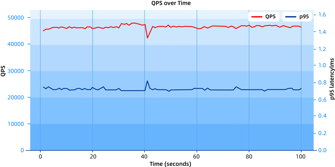
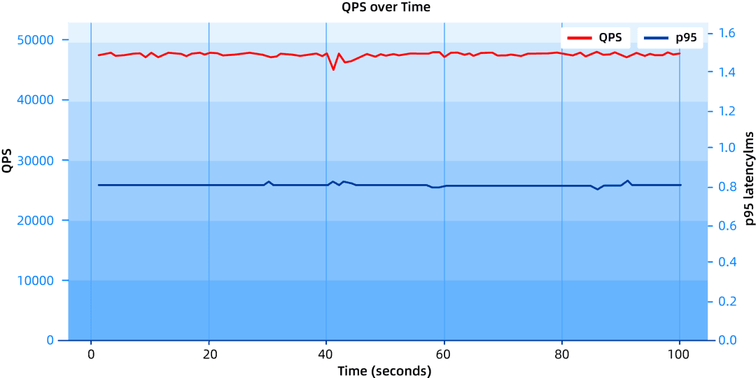
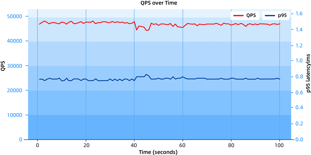
In a real production environment, there are many partitions, and only a small fraction are splitting at the same time, so the impact of splitting is even smaller.

To make automatic partitioning convenient, for certain scenarios — such as global indexes and KV scenarios like HBase — we enable splitting by default, so users can use it without any configuration. For other scenarios, users only need to set two tenant-level parameters to use automatic splitting.

Use Cases

Currently, OceanBase supports automatic partition splitting in row-store table mode, so the applicable business scenarios are mainly those suited to row-store tables, including KV scenarios and OLTP scenarios.

KV Scenarios

In OceanBase versions that did not yet support automatic partitioning, the default recommendation was to pre-partition by Key, with the number of partitions typically set to several hundred up to a thousand or more. This approach usually spreads the data volume well and supports point-lookup workloads, but it isn’t friendly to range scans because every partition must be scanned. At the same time, Key partitioning scatters old and new data together, making partition-level data management inconvenient.

Since the first phase of OceanBase automatic partitioning supports automatic Range / Range Columns partitioning, it inherits one of the advantages of Range partitioning — it suits range scans — while also having the ability, which ordinary Range partitioning lacks, to automatically split based on data volume to spread the data out. To avoid write hot spots, you should avoid appending writes by primary key under automatic partitioning. If the business has no obvious read/write hot spots along the primary key range, then even if the business workload is all point lookups, automatic partitioning can be used to spread the load.

Auto-scaling OLTP

In OceanBase versions that did not yet support automatic partitioning, to make better use of the distributed cluster, users had to design relevant partitions based on business rules to spread the data volume and workload across nodes. With automatic partitioning supported, we can make all tables automatically splitting by default. Users create ordinary non-partitioned tables at the start of the business, and as the business grows, the database itself automatically splits partitions to achieve automatic load balancing.

To help everyone better understand the applicable scenarios, here are a few examples of where automatic partitioning is used.

Smooth Business Migration

The first scenario is smooth business migration. The industry already has KV databases and distributed relational databases that support automatic splitting. Whether it’s an auto-scaling KV database or a distributed relational database, their table schemas in the source database usually have no partitions. If you want to migrate to OceanBase to enjoy advantages such as high compression and high performance, but don’t want to modify the partitioning of each table one by one, you can migrate the schema over unchanged and use automatic partitioning to take advantage of the distributed database’s capabilities, making the migration process smoother.

Load Balancing

The second scenario is making the most of the resources on each node.

There may be two cases here. In the first case, with multiple zones, each zone has only one machine, but the three zones together add up to three machines. To fully utilize these three machines, we generally use the random deployment mode, hoping to spread the load across multiple nodes. If a table has only a single partition, this can’t be achieved, because a partition can have only one Leader, so resources can’t be reused.

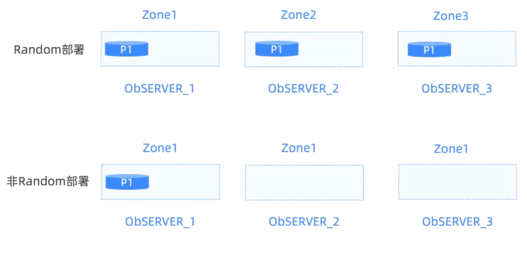
If you enable automatic partitioning for the table and it splits into multiple partitions, you can distribute the Leaders of all partitions evenly across the nodes, achieving load balancing.

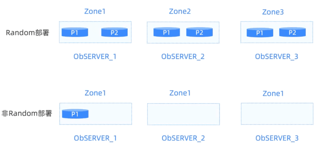
Likewise, if a zone already has multiple nodes, then even in a non-random deployment, it has the resources of multiple nodes available. In this case you can also use the splitting capability to generate multiple partitions and migrate them to different nodes for load balancing.

Automatically Handling Business Growth

We’ve encountered customers who may have many business lines and who themselves find it hard to predict which businesses will grow significantly in the future.

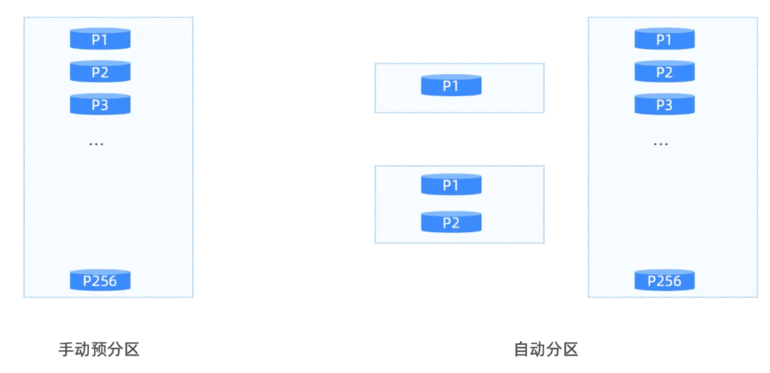
To cope with this potential growth, in the manual-partitioning era we usually advised customers to configure a relatively large number of partitions to handle future surges in data volume or business traffic. For example, configuring 256 partitions per table. When the cluster has a large amount of business data, the number of partitions becomes very large, which is suboptimal. With automatic splitting, partitions are split automatically based on each table’s data volume.

• A small business table has little data, so it won’t split and occupies few partitions.
• A large, successful business table will, as its data grows, generate a number of partitions matching the business scale, automatically handling growth.

Manual and Automatic Combined

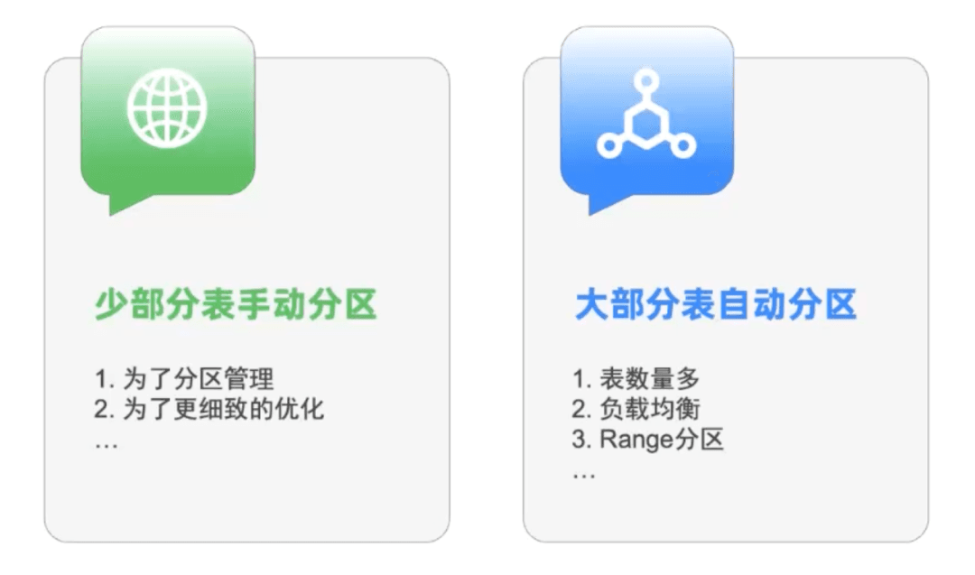
OceanBase lets you independently set whether automatic partitioning is enabled for each table. That is, you can individually choose automatic or manual partitioning per table. In some scenarios we may need manual partition management for certain tables.

For example, for business-level partition management and finer performance tuning, we can create specified partitioning rules for those tables individually, while other tables still use automatic partitioning.

In general, we recommend automatic partitioning for most tables, with only a small number of tables with special needs having manually configured partitioning rules. Overall, this also saves a lot of partitioning configuration across tables.

Automatic Splitting of Global Indexes

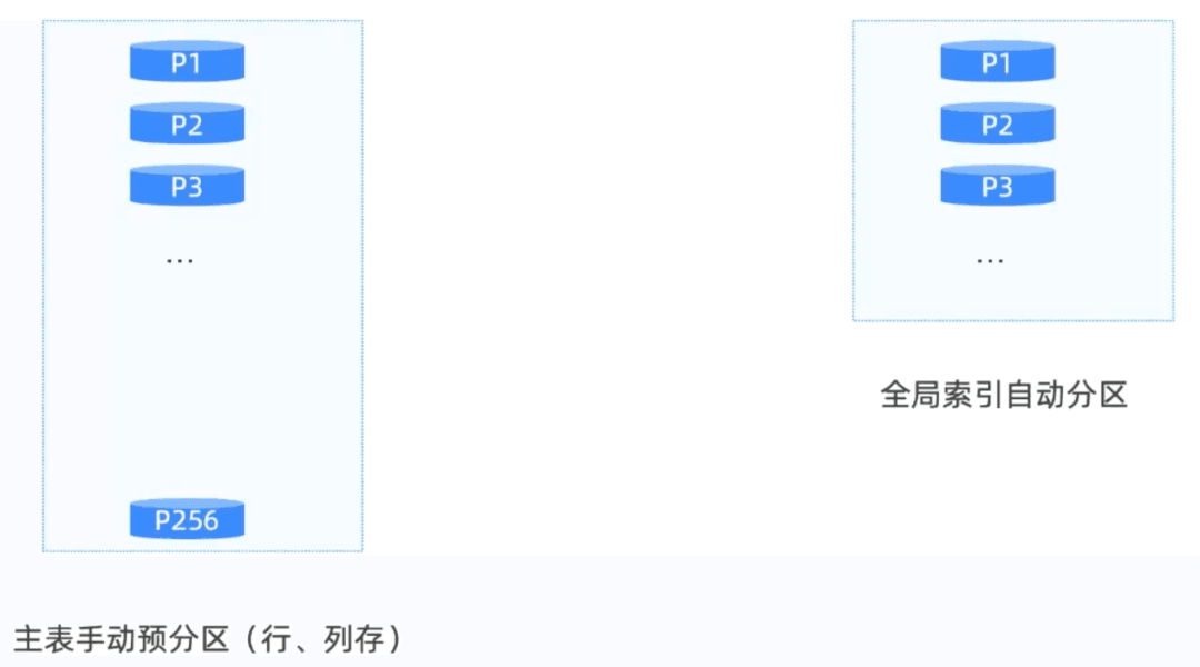
In some business scenarios, the primary table may already have been partitioned. But some queries don’t include the partition key, in which case you need to create a global index to avoid scanning all partitions.

Index queries are often range scans, so they suit Range partitioning. However, the data type of a global index’s index key is often variable, making it hard to determine the partition’s upper and lower bounds. Therefore, this case is also very well suited to enabling automatic partitioning for the global index alone. It’s particularly worth noting that even when the primary table is a column-store table, if the global index is row-store, we can still split it automatically.

Usage

Getting Started

To use the automatic partitioning feature, you only need to pay attention to two configuration items:

• enable_auto_split: A tenant-level configuration item that controls whether automatic partitioning is enabled for this tenant. Disabled by default.
• auto_split_tablet_size: A tenant-level configuration item that controls the threshold at which splitting is triggered after automatic partitioning is enabled for the tenant. The default value is 2 GB.

If you need to enable automatic partitioning and have sufficient memory resources, use ALTER SYSTEM SET enable_auto_split = true; to turn it on. Since tenant memory resources are generally limited, and the number of tablets we support is related to the tenant’s memory size, the rule-of-thumb formula is that 1 GB can allocate 20,000 tablets. So, to avoid creating too many tablets, you can adjust auto_split_tablet_size to prevent allocating too many tablets due to a large data volume.

Advanced Usage

Tenant-level configuration makes it easy to start using automatic partitioning, but this approach turns on automatic partitioning mode for all businesses within the tenant.

As just mentioned, there are also scenarios that combine manual and automatic partitioning, for example:

1. A user has a new cluster or new business that plans to adopt OceanBase and wants to try automatic partitioning on just a few tables first. This can be controlled by specifying whether to enable automatic partitioning when creating the table.

-- Create an auto-partitioned non-partitioned table (using the default 128 MB split threshold)
CREATE TABLE auto_pt2 (c1 int, c2 int, primary key(c1));
				PARTITION BY RANGE ();

-- Create an auto-partitioned non-partitioned table (split threshold of 1024 MB, user-configured)
CREATE TABLE auto_pt3 (c1 int, c2 int, primary key(c1))
				PARTITION BY RANGE () SIZE('1024MB');

2. A user has an existing OceanBase cluster that they upgrade to an OceanBase version supporting automatic partitioning and wants to try automatic partitioning on some tables. This can be controlled by modifying the automatic partitioning attribute.

-- Table t1 upgraded from an older OceanBase version, with automatic partitioning not enabled
CREATE TABLE t1 (C1 INT, C2 INT, PRIMARY KEY(C1))
		PARTITION BY RANGE(C1) SIZE('10GB')
    (PARTITION p0 VALUES LESS THAN(100),
     PARTITION p1 VALUES LESS THAN(200),
     PARTITION p_max VALUES LESS THAN (MAXVALUE)
    );
-- Change table t1 to an auto-partitioned table
ALTER TABLE t1 PARTITION BY RANGE() SIZE('128MB');

3. A user can design partitions for the primary table, but finds it hard to manually set good Range partitioning rules for the global index. This can be controlled via the global index auto-split configuration.

-- Turn on the global index auto-split configuration item
ALTER SYSTEM SET global_index_auto_split_policy = 'ALL';
-- Adding a global index on a partitioned table will automatically enable auto-splitting for the global index
ALTER TABLE t1 ADD INDEX(c1) GLOBAL;

What’s more?

The following content is prerequisite knowledge about OceanBase partitioning.

Feel free to read it selectively.

Why Can Partitioning Make Queries Faster?

On the OceanBase community forum, a very common user question is: “Can partitioning by date speed up queries?”

In my understanding, besides letting the data of one super-large table balance across different database nodes, partitioning has another purpose: accelerating queries. This is because queries use the partition key in the filter conditions to perform partition pruning.

Take the following two examples:

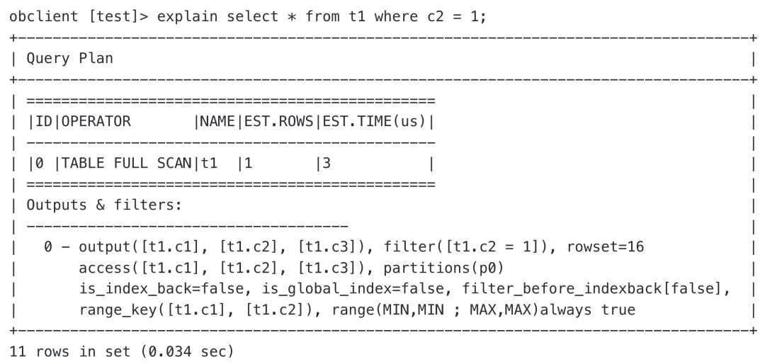
• If the filter conditions include the partition key, you can see partitions(p0) in the plan, meaning only the data in partition p0 was scanned.

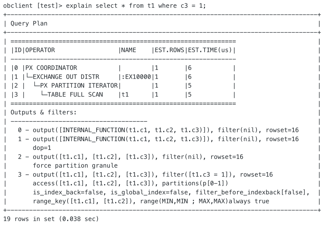
• If the filter conditions don’t include the partition key, you can see partitions(p[0-1]) in the plan, meaning the data in all partitions p0 and p1 was scanned. Here, the PX PARTITION ITERATOR operator is the iterator used to loop over and scan all partitions.

Why Must the Primary Key Include All Partition Keys?

Many community users ask: “I have an order transaction table with a lot of data, and I want to partition by year. Right now only the ID column is the primary key. When I tried, it seems I can’t partition by date. Do I have to make the date and ID a composite primary key in order to partition?”

The answer is yes — the primary key must include all partition keys.

This is because the primary key’s uniqueness check is performed within each partition. If the primary key doesn’t include all partition keys, this check breaks down. So MySQL and other databases generally have this requirement too.

-- If the primary key doesn't include all partition keys, creating the table fails with an error, and the error message is quite clear.
create table t1(c1 int, 
                c2 int,
                c3 int,
                primary key (c1))
partition by range (c2) 
  (partition p1 values less than(3),
   partition p1 values less than(6));

ERROR 1503 (HY000): A PRIMARY KEY must include all columns in the table's partitioning function

Note:

Regarding this restriction, a while back a database-world KOL argued that the statement above was too absolute, tried to come up with a counterexample, and finally found a third-party PostgreSQL extension called pg_pathman.

To improve the flexibility of partition setup, such third-party extensions don’t require the partition key to be a subset of the primary key or unique key, but this often means the primary key and unique key in the database no longer guarantee uniqueness, which can introduce serious correctness problems. Still, it does break the restriction after all.

In the end, the words “generally” were added to that statement.

Here’s an example explaining the reason:

• We create a table whose primary key is c1 and c2 and whose partition key is c2: values less than 3 go into partition p0, and values greater than or equal to 3 and less than 6 go into partition p1. Then we insert two rows: the first in partition p0, the second in partition p1.

create table t1(c1 int, 
                c2 int,
                c3 int,
                primary key (c1, c2))
partition by range (c2) 
  (partition p0 values less than(3),
   partition p1 values less than(6));
Query OK, 0 rows affected (0.146 sec)

obclient [test]> insert into t1 values(1, 2, 3);
Query OK, 1 row affected (0.032 sec)

obclient [test]> insert into t1 values(1, 5, 3);
Query OK, 1 row affected (0.032 sec)

obclient [test]> select * from t1;
+----+----+------+
| c1 | c2 | c3   |
+----+----+------+
|  1 |  2 |    3 |
|  1 |  5 |    3 |
+----+----+------+
2 rows in set (0.032 sec)

• If the primary key were only c1 without c2, then the uniqueness check on column c1 within partitions p0 and p1 would both succeed, because the values of column c1 within each partition are not duplicated (each partition has only one row, so naturally there’s no duplication within a partition). It would then determine that the inserted data satisfies the primary key constraint.

obclient [test]> select * from t1 PARTITION(p0);
+----+----+------+
| c1 | c2 | c3   |
+----+----+------+
|  1 |  2 |    3 |
+----+----+------+
1 row in set (0.033 sec)

obclient [test]> select * from t1 PARTITION(p1);
+----+----+------+
| c1 | c2 | c3   |
+----+----+------+
|  1 |  5 |    3 |
+----+----+------+
1 row in set (0.034 sec)

• But in fact there’s a duplicate value c1 = 1 across partitions, and the data does not satisfy the primary key constraint (with only column c1 as the primary key). So when partitioning, all databases require the primary key to include all partition keys.

Which Partitioning Method Should a Partitioned Table Prefer?

The advantage of a distributed database is divide-and-conquer for both storage and access problems. Access to each partition can be served by the node where that partition resides. Even if a SQL statement has very high concurrency, since it accesses different partitions served by different nodes, each node has the capacity to satisfy a certain QPS on its own, and all nodes together can deliver greater QPS. If you then scale out the number of nodes, the total QPS of that SQL also increases accordingly — this is the best case in a distributed database.

The goal of partitioning is to distribute large amounts of data and access requests evenly across multiple nodes. First, to fully utilize resources for parallel computation and eliminate query hot spots; second, to use partition pruning to improve query efficiency. If each node bears data and requests evenly, then in theory 10 nodes should handle 10 times the data volume and access of a single node. However, if partitioning is uneven, some partitions will have relatively high data volume or request volume, resulting in data skew, which can cause uneven resource utilization and load across nodes. The data concentrated in the skew is also called hot data. The most direct way to avoid hot data is to randomly assign data to nodes (with no rule) at storage time, but the downside is that at read time you don’t know which partition to look in for the record and have to scan all partitions, so this approach isn’t very meaningful. The partitioning strategies actually used in practice all follow certain rules.

Users must plan partitioning based on real business scenarios, with clear business query conditions; don’t apply arbitrary partitioning rules when the scenario is unclear. When planning partitions, it’s recommended to keep the data volume of each partition relatively balanced.

The three most commonly used partitioning methods are as follows:

• HASH partitioning: Generally suitable when the partition column has a large NDV (number of distinct values) and is hard to divide into clear ranges. The advantage is that it easily distributes data without a specific rule evenly across partitions; the disadvantage is that partition pruning is hard to apply during range queries.
• RANGE partitioning: Generally suitable when the partition key can be easily divided into clear ranges. For example, a large table recording transaction information can be RANGE-partitioned by the column representing the information’s timestamp.
• LIST partitioning: Generally suitable when you need to explicitly control how each row maps to a specific partition. The advantage is that you can precisely partition unordered or unrelated datasets; the disadvantage is that partition pruning is hard to apply during range queries.

To better support parallel computation and partition pruning, OceanBase also supports secondary (sub)partitioning. OceanBase’s MySQL mode currently supports six partition types — HASH, RANGE, LIST, KEY, RANGE COLUMNS, and LIST COLUMNS — and a secondary partition is a combination of any two partition types.

For example, in the user billing domain, the database often needs to do HASH primary partitioning by user_id, and then within each primary partition, continue with RANGE secondary partitioning by bill creation time.

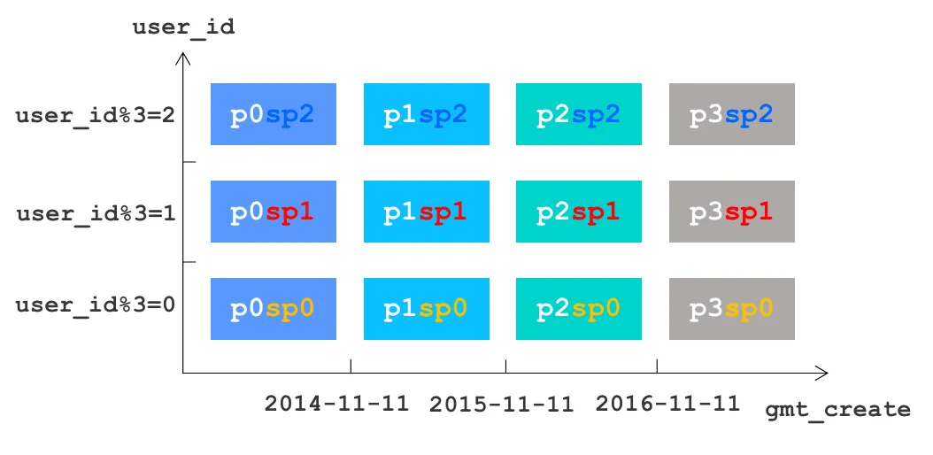
Although OceanBase supports both RANGE + HASH and HASH + RANGE combinations for composite partitioning, for RANGE partition add/drop operations, RANGE must be the primary partition. So for transaction tables with large data volumes, for easier maintenance (adding and removing partitions), it’s recommended to use the RANGE + HASH combination (time column as RANGE primary partition + business column as HASH secondary partition).

To summarize:

• For partitioning, prefer a time column as RANGE primary partition + a business column as HASH secondary partition.
• Otherwise, design partitions based on the data clustering dimension and common query statements.

Adapted from an article on the OceanBase community WeChat account: OceanBase PoC Lessons (Part 2) — AP Workloads

How to Perform Manual Partition Splitting?

OceanBase supports manually splitting partitions (REORGANIZE) in a partitioned table, that is, splitting an existing partition into multiple partitions. This feature lets you specify the partition to split and the split points for the new partitions, then manually execute the partition split command to adjust partitions based on your needs and data growth.

OceanBase currently (version 4.4.0 and below) only supports manual partition splitting on primary-level Range / Range Columns partitioned tables.

Example:

• Create a Range-partitioned primary-level table test_tbl1.

CREATE TABLE test_tbl1(col1 INT, col2 INT, PRIMARY KEY(col1))
    PARTITIONBYRANGE(col1)
    (PARTITION p0 VALUESLESSTHAN(100),
     PARTITION p1 VALUESLESSTHAN(200),
     PARTITION p2 VALUESLESSTHAN(300),
     PARTITION p_max VALUESLESSTHAN (MAXVALUE));

• Split partition p0 of table test_tbl1 into three new partitions, with split points at the rows corresponding to the values 30 and 60. After splitting, the original partition p0 is divided into three new partitions: p0_1, p0_2, and p0.

ALTER TABLE test_tbl1
    REORGANIZE PARTITION p0 INTO (
        PARTITION p0_1 VALUES LESS THAN (30),
        PARTITION p0_2 VALUES LESS THAN (60),
        PARTITION p0 VALUES LESS THAN (100));

• Split partition p_max of table test_tbl1 into three new partitions, with split points at the rows corresponding to the values 400 and 500. After splitting, the original partition p_max is divided into three new partitions: p_max_1, p_max_2, and p_max_3.

ALTER TABLE test_tbl1
    REORGANIZE PARTITION p_max INTO (
        PARTITION p_max_1 VALUES LESS THAN (400),
        PARTITION p_max_2 VALUES LESS THAN (500),
        PARTITION p_max_3 VALUES LESS THAN (MAXVALUE));

• View the structure and definition of table test_tbl1.

SHOW CREATE TABLE test_tbl1 \G

The result returned is as follows:

*************************** 1. row ***************************
       Table: test_tbl1
Create Table: CREATE TABLE `test_tbl1` (
  `col1` int(11) NOT NULL,
  `col2` int(11) DEFAULT NULL,
  PRIMARY KEY (`col1`)
) ORGANIZATION INDEX DEFAULT CHARSET = utf8mb4 ROW_FORMAT = DYNAMIC
 partition by range(col1)
(partition `p0_1` values less than (30),
partition `p0_2` values less than (60),
partition `p0` values less than (100),
partition `p1` values less than (200),
partition `p2` values less than (300),
partition `p_max_1` values less than (400),
partition `p_max_2` values less than (500),
partition `p_max_3` values less than (MAXVALUE))
1 row in set (0.003 sec)

Finally, I’d like to recommend the WeChat official account “Lao Ji’s Tech Talk” run by Lao Ji, the OceanBase open source lead. It continuously publishes all kinds of technical content related to #Databases, #AI, and #Tech Architecture. Friends who are interested are welcome to follow!

“Lao Ji’s Tech Talk” hopes not only to keep bringing you valuable technical insights, but also to contribute to the open source community together with you. If you appreciate the OceanBase open source community, please light up a little star ✨! Every Star you give is motivation for our efforts.