OceanBase PoC Lessons Learned (Part 2) — AP Workloads

Background

A while ago, the OceanBase community WeChat account reposted “OceanBase PoC Lessons Learned (Part 1)” by the renowned Qingtao, introducing the wealth of OceanBase PoC experience he has accumulated. However, Qingtao is extremely busy, and the SQL-related PoC article he previously teased is still being polished.

Good food is worth the wait, but I figured I’d serve up an appetizer on Qingtao’s behalf—a humble follow-on to his work.

This summary of PoC experience for OceanBase AP workloads is based on notes I took during a related tech talk given by the esteemed Baihua. It focuses mainly on business migration and database object design, and won’t touch much on operations.

PoC (Proof of Concept) means:

A process or practice for verifying whether a given theory or solution is feasible.

Its main purpose is to demonstrate, through a simple, fast, and low-cost implementation, whether a given framework, technology, solution, or project can achieve the expected goals—confirming feasibility or exploring potential application scenarios.

Today I’m sharing these study notes on the community WeChat account, hoping they help OceanBase Community Edition users avoid a few pitfalls during their PoCs. Without further ado, let’s begin.

Migration Strategy

The OceanBase AP scenario PoC we’re discussing this time is about replacing an existing AP system. In other words, the premise is that the schema model and other aspects of the original business database have already been validated, rather than being designed from scratch for a new business.

Overall, you can adopt a straight-migration strategy: if the original system uses row storage, it stays row storage after replacing it with OB; if the original system uses columnar storage, it stays columnar after replacement. The clustering key, partition key, and so on can also be kept consistent with the original system. Only after identifying special cases should you introduce inconsistent designs.

Indexes are the one exception here—they’re not a fully one-to-one replacement. Some AP databases may create indexes rather casually, in enormous numbers. In OceanBase, indexes should be created as much as possible based on actual business needs, keeping only the indexes you need during the replacement.

Schema Design

Here’s a table listing some key points to watch when designing schemas across mainstream AP databases.

The contents of the table are incomplete and may be further refined and revised in later study notes. The table just lists some information, mainly to help translate terminology between different databases.

	OceanBase	Other AP DataBases
Data Clustering	- Heap table: insertion order - Index-organized table: primary key order	- CLUSTERED KEY - ORDER BY - CLUSTER ON
Data Distribution	- Partitioning   - Typically a level-1 time-dimension range partition   - A level-2 hash partition - tablegroup sharding - primary zone - Replicated tables	- DISTRIBUTED BY   - HASH / RANDOM / ROUNDROBIN / REPLICATED - BROADCAST
Compaction Strategy	- Manual compaction - table_mode:   - normal   - queuing   - moderate   - super   - extreme	- None - Manual compaction
Partition Management	- Manual partitioning - Set a partitioning plan in ODC - 435 BP2 automatic partition splitting - 435 BP2 dynamic partition management	- LIFECYCLE - TTL (partition_retention_condition) - Dynamic partition management
colocate	tablegroup	colocate_with
Aggregation Table	Alternative MV	- Aggregation Table - Alternative MV
Smallest Migration Unit	partition / tablet	- shard - tablet - share storage - segment

The table above is too large to read comfortably on a phone, so let me briefly record the key points from it in text below.

Data Clustering

Most AP databases use heap tables clustered along the time dimension (from old to new), which corresponds to heap tables in OceanBase. If another AP database uses a CLUSTERED KEY, that corresponds to OceanBase’s index-organized table (the default). In OceanBase, you can use the default_table_organization configuration item to control whether a created table is a heap table or an index-organized table by default.

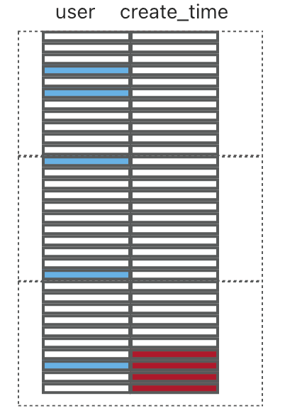
Here is an illustration of a heap table and an index-organized table (blue indicates data belonging to one specific user, red indicates data belonging to one day).

• Clustered by time (heap table default):

• Clustered by user (index-organized table, primary key is user):

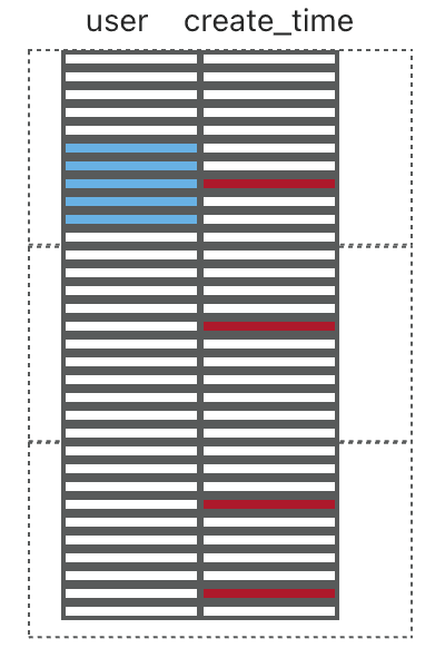
• Clustered by time + partitioning:

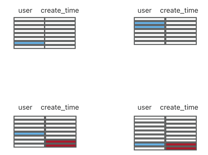
Among common AP databases, some cluster data via a clustered key, while a few use relatively complex clustering schemes that span many levels. Because different databases may cluster data somewhat differently, directly migrating an index from some AP database into OceanBase as a primary key may not be appropriate. You first need to understand the original database’s data clustering scheme and how its shards are split across multiple machines; otherwise, problems may arise.

Data Distribution

Data distribution here can be understood simply as how to distribute data across multiple machines. Except for share-storage databases, all of them need to consider data distribution.

Many AP databases have both partitioning (partition) and data distribution (distributed key). Partitioning is used for data management—for example, you can drop the partition that holds data older than three years. Data distribution is designed separately. When the original database’s table has both a partition and a distributed key, you need to design a partition key for the corresponding table in OceanBase. You can refer to the original database for the partitioning scheme—for example, partition by corresponds to the level-1 partition, and distributed by corresponds to the level-2 partition.

Here’s a very typical AP schema design: a heap table (4.3.5.1 OLAP mode defaults to heap tables) + a level-1 range partition on the time dimension + a level-2 hash partition on the business dimension.

In OceanBase, besides partitioning, there are also concepts such as tablegroup, replicated tables, and primary zone, which I won’t explain one by one here.

Compaction Strategy

What you need to understand here is OceanBase’s adaptive compaction optimization configuration for buffer tables; see “In OceanBase, How Do You Address the Read Amplification Problem of the Storage Engine?”

The title of the WeChat article above was poorly chosen and a bit off-topic, but by the time I wanted to change it, it was already too late. It actually introduces the five different levels of compaction strategy in the table-level configuration item table mode.

Partition Management

For OceanBase’s partition management, the most common approach is usually to set partitions manually. In AP scenarios, the most common setup is the level-1 range partition (time dimension) plus level-2 hash partition mentioned above.

Beyond that, OceanBase also has some automatic partitioning capabilities:

• Set a partitioning plan in ODC
• 435 BP2 automatic partition splitting
• 435 BP2 dynamic partition management

In the past, the more common approach was to automatically create and clean up partitions via ODC.

Now, in version 435 BP2 and above, the kernel directly supports automatic partition splitting and dynamic partition management. (Going forward, the kernel R&D team will continue to publish technical content on automatic partition splitting and related topics on this WeChat account, and will also introduce these features in detail through community activities such as hands-on online sessions and live streams.)

Collation

In AP scenarios, the recommendation is to set the collation of string-type fields in the business to binary wherever possible—for example, COLLATE = utf8mb4_bin. Because binary directly compares the binary representation, there’s no need to consider issues like case sensitivity during comparison, so it’s much more efficient than the comparison methods of other collations. This is easy to understand.

I’ve also written some optimization code for string expressions in OceanBase, so I know that many string-related operations in the kernel have various short-circuit optimizations that take effect only for binary, which can further improve performance.

As you can also see in the table above, many mainstream pure-AP databases support only utf8 binary, because the logic is simple, the efficiency is high, and it’s easier to optimize with all sorts of tricks. If they do support other collations, the default is generally case-insensitive.

This point may be small and oft-repeated, but it’s important. Some of OceanBase’s AP users could have used binary for collation, but set it to something else instead, such as xxx_general_ci. Changing it after going live becomes very troublesome: re-sorting data is generally an Offline DDL, the time it takes is tied to the data volume, the duration is unpredictable, and you can only do it outside business hours. So try to set the collation correctly from the very beginning.

Indexing

Indexes in OceanBase may differ from those in pure-AP databases: within a single table scan operator, predicate filtering on the same table can use only one index. So the recommendation is to create indexes on demand, and try not to create large numbers of (unnecessary) indexes the way some pure-AP databases do.

OB is adding index merge capability, which splits the query predicate so that each part of the predicate uses a different index for an index range scan, then merges the scan results from the various index tables before performing a unified table lookup. When the individual indexes in a query are not very selective but their combined selectivity is strong, this offers a significant performance advantage.

Current versions already support index merge via the UNION_MERGE hint. As AP workloads continue to expand, OB will soon also support index merge across multiple full-text indexes and secondary indexes, which is more commonly needed.

colocate / tablegroup

When spreading out data, some AP databases support adjusting the distribution of data across different nodes at a finer granularity. For example, StarRocks supports colocate_with, which can set the partition distribution rules of two or more tables to be consistent, thereby significantly reducing the data redistribution overhead in distributed queries and improving Join query performance.

Other pure-AP databases don’t support this capability; most have a very simple distributed by distribution key. But as long as you can keep the hash partition rules and the number of shards consistent, the distribution rules will generally be the same.

In OceanBase, you can use tablegroup to replace a capability similar to colocate_with. A tablegroup is also used to adjust the partition distribution rules of a batch of tables, so that queries involve as little data redistribution over the network as possible, making partition-wise joins appear more often in the plan.

Complex Data Types

The complex data types commonly used in AP scenarios are json, bitmap, array, and string. OceanBase supports all of these, so you can migrate them directly—I’ll skip them for now.

Aggregation Table

Currently only StarRocks has this Aggregation Table. In OceanBase, you can use materialized views instead.

Smallest Migration Unit

Here, each database generally just uses a different name—some call it a shard, some a segment, some share storage—and there’s really no need to dwell on it. The smallest migration unit in OceanBase is logically called a partition, and the physical shard corresponding to a partition is called a tablet. That’s all you need to know.

Summary of Schema Design for AP Scenarios

Considerations for schema design in OceanBase AP scenarios:

1. Data clustering dimension: usually by time, and by user ID in some scenarios. In certain scenarios you also have to consider the impact of incremental data on compaction—for example, by clustering along the time dimension, you can try to cluster incremental data together, which increases query efficiency and improves compaction speed.
2. Row storage / columnar storage: keep it consistent with the original system as much as possible, and only introduce inconsistent designs after identifying special cases.
3. Incremental data: if you partition along the time dimension and mainly update recent data, you should try to cluster the incremental data together. If the original table has no partitioning, you can also use hash partitioning to spread the incremental data across multiple machines, fully leveraging multi-machine performance.
4. Partitioning: columnar storage increases the complexity of managing data within a partition, so compared with row storage, it should use fewer partitions. AP scenario recommendation: set the number of hash partitions to half the CPU count of a single zone, keep the number of partitions per machine below 100,000, and keep the number of rows per partition above 1 million.
5. table mode: use queue table mode for identified buffer tables.
6. collation: use utf8mb4_binary wherever possible—performance generally improves by 20%–30% after the switch.
7. Indexing: in AP scenarios, try to avoid optimizing with index creation; based on the indexes already present in the original system, create a small number of necessary indexes on demand.
8. Replicated tables: they affect write performance, so use them only as needed.

The Respective Advantages of Row Storage and Columnar Storage

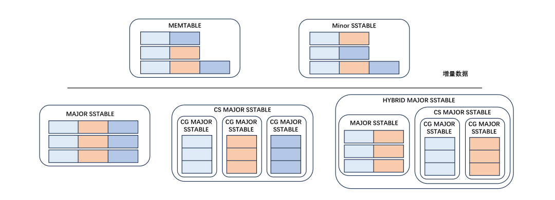
For the implementation of columnar storage, you just need to know these two things:

• Only the baseline data (major sstable) is columnar. The incremental data memtable and the dumped sstables are all row storage.
• In hybrid row-column storage, the row-format incremental data is shared.

Advantages of columnar storage:

• For wide tables, scanning only a subset of columns saves IO.
• High compression ratio (compared with row storage).
• Skip index is available by default, enabling fast filtering (row storage requires creating it manually).

Advantages of row storage:

• Suitable for point lookups / small-range scans (operations that need to fetch the complete row, such as insert on duplicate update, index table lookups, and NLJ).
• Queries can be accelerated via the row cache.
• Fast compaction (during compaction, there’s no need to convert incremental and baseline data between row and column formats). For columnar storage, you can appropriately increase the number of merge threads via merge_thread_count. You also need to watch IO—for example, you can consider increasing _io_read_batch_size and decreasing _io_read_redundant_limit_percentage.

To be continued:

The topic of row storage vs. columnar storage is too big, so this time I’ll cover just a few of the most basic points; the rest will be discussed in detail in the next PoC study notes.

Common Problems with Incremental Data

Common problems:

1. If the incremental data is scattered, causing all the baseline data to be modified along with it, this leads to a fairly serious write amplification problem. Combined with the slow columnar compaction issue, it can make compaction take too long. For tables organized and updated along the time dimension, this is generally not a problem.
2. The incremental data itself is slow to query: single row, no pushdown, no encoding. If the incremental data is all in memory, that’s fine, but if there are dumped incremental sstables, since they are row storage, there may be row-column conversion overhead as well as extra IO overhead.
3. Query “drag”: this has the biggest impact. For example, a single incremental row may drag down the query performance of the 100–1,000 rows before and after it. Because as long as one row in a microblock has been modified, querying the entire microblock may degrade to single-row iteration, hurting performance. This problem will be optimized away soon.

Solutions:

1. Control the scope of write amplification by choosing the range partition size. For example, if you originally partitioned by month, in OceanBase you might be able to switch to partitioning by week to reduce the impact of write amplification.
2. For tables that originally had no partitioning, in OceanBase you can consider using hash partitioning to spread the incremental data across multiple machines, fully leveraging the multi-machine hardware resources.
3. Adjust the table mode to speed up compaction, and try to query the incremental data only after compaction is complete.
4. Adjust the data clustering scheme to cluster the incremental data together, avoiding queries being “dragged down” everywhere.

Summary of OceanBase AP Scenario PoCs

The following applies to OceanBase 435 bp2.

• Choose the OLAP tenant template, with defaults: columnar storage, heap tables, auto dop, utf8mb4_binary, NLJ off, etc.
• When the original database has a clustered key / clustering_key / order by or other clustering index, it is usually no longer clustered along the time dimension. You need to use an index-organized table (you can’t use a heap table) and design a primary key to achieve a similar effect.
• Keep row storage / columnar storage consistent with the original system—for example, row storage when migrating from MySQL, columnar storage when migrating from some pure-AP database, and hybrid row-column storage when migrating from MySQL + some AP database (this will be discussed in detail in a later PoC study note).
• For partitioning, prioritize: heap table + level-1 range partition on the time column + level-2 hash partition on the business dimension. Otherwise, design partitions based on the data clustering dimension and the common query statements.
• Use utf8mb4_bin for collation wherever possible.
• Incremental data problems: cluster the incremental data together + adjust the table mode.
• Trade space for time: a small number of indexes on demand + materialized views.
• Bypass import: bypass import takes a table lock, which affects DML operations (this will be discussed in detail in a later PoC study note).