A Quick Introduction to Vector Databases

Vector databases have become essential in the AI era, and many people around me have started sharing knowledge on the topic.

A couple of days ago, I read an article by Mr. Hongbo published on the Lao Ji WeChat account: “The Key Path and Application Cases of OceanBase Supporting AI at Scale”. I learned quite a few new things from it. However, the article mentioned many specialized terms. You need some background knowledge in AI and databases to fully understand it.

Today, I focused on studying those new terms and made some quick notes. I’m sharing them here. This article has no prerequisites. It’s written in plain, easy-to-understand language, perfect for a “gentle first look” at vector databases. If you want to go deeper afterward, this article can serve as a solid starting point.

Here are the fundamental vector database concepts I’ll explain:

1. Embedding
2. Distance / similarity metrics
   • Cosine_distance
   • Inner_product
   • L1_distance
   • L2_distance
   • Jaccard Distance
   • Hamming distance
3. Similarity search algorithms
   • Typical algorithms
     • Inverted index + data compression
     • Navigation graph index + distributed
   • HNSW
   • IVF
   • DiskANN
4. Index compression algorithms
   • SQ (Scalar Quantization)
   • PQ (Product Quantization)
5. Recall

Let’s get started.

The concept of a vector database has been discussed extensively by now. Put simply: in a vector database, you use multi-dimensional vectors to store the features of certain objects. By computing the positional relationships between vectors in space, you can determine how similar those objects are.

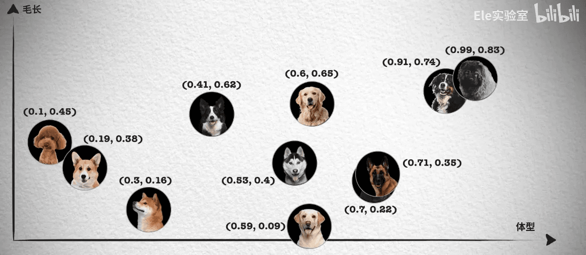
• An object can have multiple orthogonal features extracted from it, such as body size and fur length. Each feature represents one dimension of the vector.
• The finer the precision of each dimension, the greater the discriminative power.
• The more dimensions there are, the greater the discriminative power, and the more precise the query becomes.
• For example, our structured data is computed in a one-dimensional space. The higher the dimensionality, the larger the computation and query space, and the greater the computational cost.

Embedding

Embedding is the process of using a deep-learning neural network to extract content and semantics from unstructured data—turning images, videos, and other media into feature vectors.

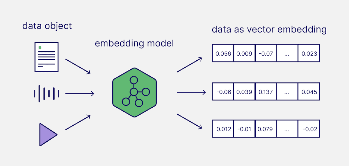
Embedding techniques map original data from a high-dimensional (sparse) space to a low-dimensional (dense) space. This converts feature-rich multimodal data into multi-dimensional arrays (vectors). You can then compute vector distances to determine the similarity of the original multimodal data.

Distance / Similarity Metrics

Common ways of measuring similarity involve some basic middle-school math: cosine similarity, inner product (dot product), Euclidean distance, and Manhattan distance. Let’s review them together and reminisce about our bygone youth. The following content references the OceanBase official documentation “Vector Functions”.

Cosine_distance

Cosine similarity computes the cosine of the angle between two vectors. When two vectors point in the same direction, the cosine similarity is 1. When the angle between them is 90 degrees, the cosine similarity is 0. When they point in completely opposite directions, the cosine similarity is -1.

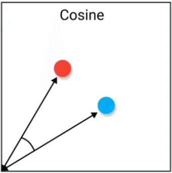
Since a cosine similarity value closer to 1 indicates greater similarity, cosine distance (or cosine dissimilarity) is sometimes used to measure the distance between vectors. You can compute cosine distance by subtracting the cosine similarity from 1.

The range of cosine distance is [0, 2], where 0 indicates an identical direction (no distance) and 2 indicates a completely opposite direction.

Inner_product (IP / Inner Product)

The inner product, also known as the dot product or scalar product, is an important operation in linear algebra. It defines a type of product between two vectors. Geometrically, the inner product captures both the directional relationship and the magnitude relationship between two vectors.

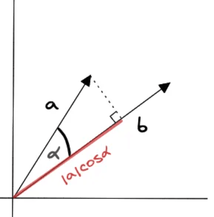
Like cosine similarity, the inner product is affected by the angular relationship between vectors. However, it’s also affected by vector length. If you normalize the vectors (divide each vector by its own length to obtain a unit vector of length 1), the inner product reflects only direction, not magnitude. At that point, the inner product becomes equivalent to cosine similarity.

L1_distance

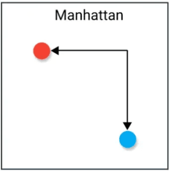
Manhattan distance computes the sum of the absolute axis distances between two points in a standard coordinate system.

A picture is worth a thousand words. The sum of the two line segments in the figure below represents the Manhattan distance between two vectors in a multi-dimensional coordinate system. It’s also known as the city-block distance.

L2_distance

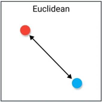
Euclidean distance reflects the straight-line distance between the coordinates of two vectors. This should be easy to understand: the red line in the figure above represents the Euclidean distance between two vectors in a multi-dimensional coordinate system.

Summary

• Cosine (cosine distance): Measures similarity by computing the cosine of the angle between two vectors. Range is [-1, 1]; the closer to 1, the more similar.
• IP (Inner Product): Computes similarity by multiplying corresponding elements of two vectors and summing them. The larger the inner product value, the higher the similarity. Commonly used in natural language processing (NLP).
• L1 (Manhattan distance): The sum of absolute differences across each dimension of two vectors. Unlike Euclidean distance, Manhattan distance focuses on differences in each dimension rather than direction.
• L2 (Euclidean distance): The straight-line distance between two vectors, expressed as the square root of the sum of squared differences across each dimension. The smaller the Euclidean distance, the more similar the vectors. Commonly used in natural language processing (NLP).

What’s more?

Next, let me introduce two common similarity metrics for binary vectors.

A binary vector is one in which each element is either 0 or 1. Binary vectors are implemented differently from floating-point vectors. To save space, databases often implement binary vectors using bytes rather than floats internally.

Jaccard Distance

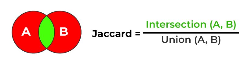
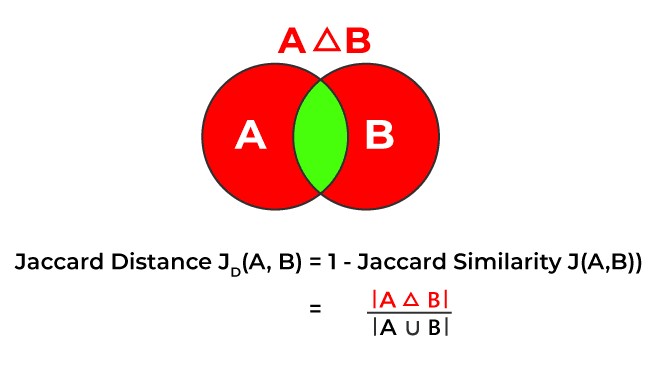
The Jaccard distance computes the proportion of elements in the union of two sets that do not belong to their intersection. It reflects the degree of difference between sets.

Hamming distance

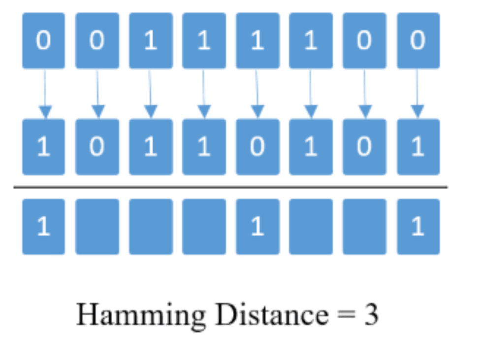
The Hamming distance is a concept from error-control coding in data transmission. It represents the number of positions at which the corresponding bits of two words differ. It’s defined as the number of 1-bits after XORing the two words together.

Similarity Search Algorithms

Vector database similarity search is a technique that quickly finds the data most similar to an input vector. It does this by computing the similarity between the input vector and target vectors. The most representative approaches are Approximate Nearest Neighbor (ANN) search and clustering-based search, exemplified by K-Means.

Typical Algorithms

Inverted Index + Data Compression

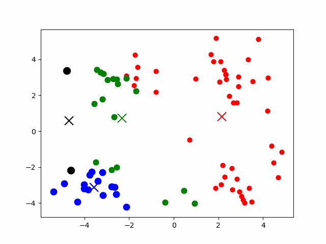
A clustering algorithm (commonly K-Means) divides the data into several clusters. It then builds an inverted index keyed by cluster centers. On each search, you first compute the similarity to the cluster centers, select the most similar cluster, and search further within it.

Navigation Graph Index + Distributed

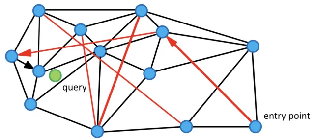
Treating vectors as nodes and vector similarities as edges, you build an approximate nearest-neighbor graph. You then perform greedy search on the graph to approach the neighbor region. Graph indexes are most efficient in memory, but they consume a great deal of it. They often rely on partitioning and distributed approaches to handle large data volumes. The downside is high cost. The upside is the ability to achieve high recall and low latency. The idea is similar to the six degrees of separation theory: through at most six people, you can connect to any stranger.

HNSW

Hierarchical Navigable Small World. A small-world graph is a graph structure that lies between a regular graph and a random graph. Its characteristic is that each node connects to only a small, limited number of nodes, and these nodes have a certain degree of clustering. Most nodes in a small-world graph are not directly connected to each other, yet most can be reached in just a few steps.

HNSW is built on the core idea that “a neighbor’s neighbor is likely also a neighbor.” Social networks are a typical small-world graph structure. Let’s first look at a data structure everyone is more familiar with—the SkipList.

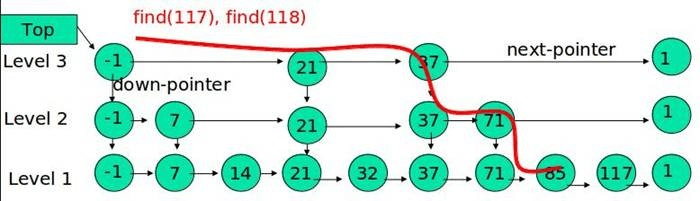
A skip list is a classic case of trading space for time. The index is divided into several levels. The bottom level (Level 1 in the figure) stores all the data, while the levels above store indexes pointing to certain data items. The higher you go, the fewer indexes there are.

The purpose of a skip list is to quickly get close to the vicinity of the point you’re searching for, and then search precisely. This avoids wasting time on pointless work along the way. As I understand it, HNSW simply applies the skip list concept to a graph structure.

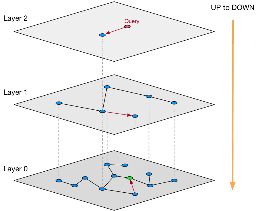
Each level of the skip list is itself a small-world network. The bottom level (Layer = 0) is a complete NSW (Navigable Small World network), while the other levels store pointer indexes pointing to graph nodes. The reason for using something like a skip list is simple: to avoid wasting time on pointless work.

The upper-level small-world graphs can be seen as scaled-down versions of the lower levels. The point of the multi-layer graph approach is to reduce the number of distance computations and comparisons during search. When retrieving, you start from the topmost (i.e., sparsest) layer. The retrieval result obtained at each layer then serves as the input to the next layer, iterating down to the final layer. In the end, you obtain the K nearest neighbors of the query point.

HNSW is currently the most popular vector retrieval algorithm. It offers fairly good performance and recall, but it has a strong dependence on memory.

IVF

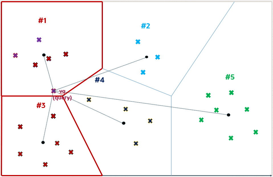
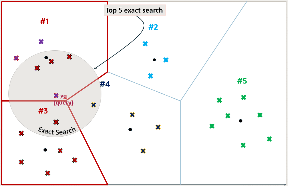
The IVF (Inverted File Index) divides the vector space into multiple subspaces via a clustering algorithm. It builds an index for each subspace. During the search, the IVF index first finds the subspace to which the query vector belongs (the red box in the figure below indicates a subspace), and then performs an exact search within that subspace.

The advantage is fast search speed. The disadvantage is suboptimal recall. Because the cluster centers are pre-built, importing incremental data does not affect the distribution of cluster centers. After data updates, you need to rebuild the clusters.

DiskANN

The problems it aims to solve:

• How can we reduce the frequency of disk access? Access memory first, and only access disk when the original vector is truly needed.
• How should we organize the data structure? Ensure that a single disk read can retrieve the relevant node and edge-graph information.

The idea behind DiskANN:

• The DiskANN algorithm combines two classes of algorithms: clustering-compression algorithms and graph-structure algorithms.
• The algorithm works as follows:
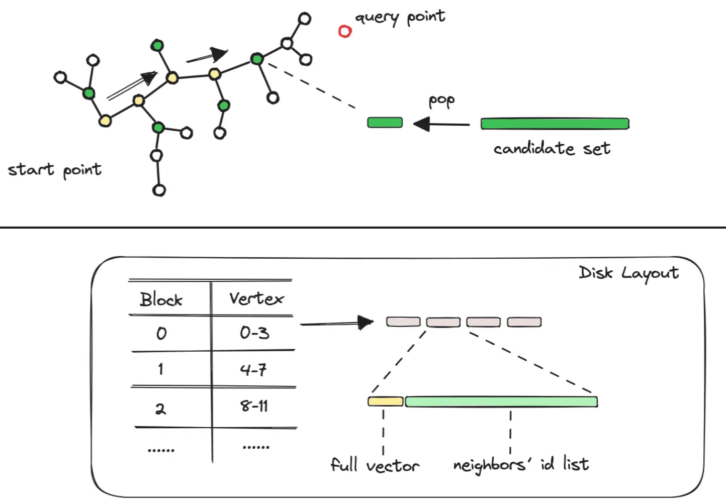
  • By compressing the original data, only the compressed codebook information and the center-point mapping information are kept in memory. The original data and the constructed graph-structure data are stored on disk. They are read from disk only when the query matches a specific node.
  • The arrangement of the vector data and the graph structure is modified so that a data point and its neighbor nodes are stored side by side. This way, a single disk operation can complete the reading of a node’s vector data, adjacent nodes, and other information.

The pros and cons of the DiskANN algorithm are both quite obvious:

• Pros: Greatly improves the read efficiency of vector recall, reduces the memory footprint of graph algorithms, and improves recall.
• Cons: The index-construction overhead is relatively high, making it better suited for static datasets (or datasets that don’t change frequently).

Index Compression Algorithms

Quantization combines existing indexes (such as IVF and HNSW) with compression methods to reduce memory footprint and speed up search.

Vector compression is generally based on reducing vector dimensionality and lowering the precision of vector elements. It falls into two categories: Scalar Quantization (SQ) and Product Quantization (PQ). For example, IVF-PQ and HNSW-PQ.

SQ (Scalar Quantization)

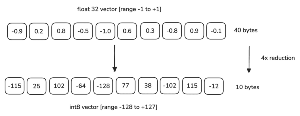
The idea is to take a high-precision floating-point vector, deliberately discard some of its precision, and turn it into a low-precision vector. This reduces computation and storage overhead. For example, replacing the elements 0.1192 and 0.1365 in a vector with a uniform 0.1.

Roughly how it works:

1. Range partitioning: First determine the approximate range of the values in the vector. Then divide this range into a number of equally spaced segments or buckets (this is called the quantization level or quantization step).
2. Value mapping: Map each element in the original vector to the nearest bucket. Specifically, round each floating-point value to the center value of its nearest quantization level—a process usually called quantization.
3. Encoding: The values mapped into each bucket can be represented in a more compact form. For example, the bucket index (an integer) is used in place of the original floating-point number, thereby achieving compression.

PQ (Product Quantization)

The idea is to reduce the dimensionality of the high-dimensional vector space. The storage and computation overhead of low-dimensional vectors is far lower than that of high-dimensional ones.

Roughly how it works:

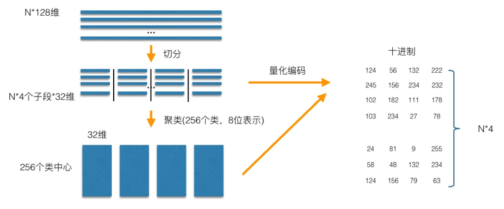
1. Dimension Splitting: First, the original high-dimensional vector space is split into multiple subspaces. Usually, a d-dimensional vector is divided into m equally sized subsets, each containing d/m dimensions. The purpose is to break a complex high-dimensional problem down into multiple lower-dimensional problems for easier handling.
2. Codebook Generation: For each subspace, build a codebook. A codebook is a set of k vectors that are the cluster centers of all training vectors within that subspace. This step is usually done via a clustering algorithm, with the vectors in each subspace assigned to their nearest cluster center.
3. Encoding: For each high-dimensional vector, compare its projection in each subspace against the corresponding codebook. Find the nearest codebook vector and record that vector’s index within the codebook. In this way, the original high-dimensional vector is converted into a sequence of integers of length m, each ranging from 0 to k-1, yielding a compact quantized representation.

Recall

Finally, let’s cover one more concept that everyone can easily grasp: recall.

Recall refers to the proportion of results in the returned result set that are close to the target vector. Recall = true positives / (true positives + false negatives).

Brute-force search can achieve 100% recall, but it’s essentially unacceptable in practice. Search based on vector indexes generally has a recall below 100%. It is an approximate, inexact search. Recall is related to the organization algorithm of the vector index, the compression algorithm (compression essentially reduces computational overhead by lowering precision), and other factors.