Spanner: Google’s Globally Distributed Database

Summary

Spanner is Google’s scalable, multi-version, globally-distributed, and synchronously-replicated database. It is the first system to distribute data at global scale and support externally-consistent distributed transactions. This paper describes how Spanner is structured, its feature set, the rationale underlying various design decisions, and a novel time API that exposes clock uncertainty. This API and its implementation are critical to supporting external consistency and a variety of powerful features: non-blocking reads in the past, lock-free snapshot transactions, and atomic schema changes across all of Spanner.

Spanner is Google’s scalable, multi-version, globally distributed, and synchronously replicated database. It is the first system to distribute data at global scale and support externally consistent distributed transactions. This paper describes Spanner’s structure, its feature set, the rationale behind its various design decisions, and a novel time API that exposes clock uncertainty. This API and its implementation are critical to supporting external consistency and a variety of powerful features: non-blocking reads in the past, lock-free snapshot transactions, and atomic schema changes across all of Spanner.

1. It is a global database, with data distributed to datacenters worldwide (able to span continents). The design goal is to support millions of machines across hundreds of datacenters, with the data volume scaling to trillions of database rows.
2. It uses Paxos to guarantee high availability of data.
3. Data can be automatically resharded during scaling up/down, data changes, or failover.

Technical Overview

1. The earliest user was F1, which uses 5 replicas. Typically this is 3 to 5 datacenters within a single geographic region, which can withstand 1–2 datacenter disasters, and reads preferentially choose the local region.
2. The initial pain points came from Bigtable:
   3. Complex, continuously evolving schemas
   4. Strong consistency in cross-region (low-latency) environments
   5. There were some attempts to use Megastore (300+ applications, such as Gmail, Picasa, Calendar, Android Market, AppEngine). Although its write throughput was rather poor, it supported a semi-relational data model and strong synchronization.
3. It began evolving from a KV store like Bigtable into a database that supports multi-version data.
   7. Data uses semi-structured tables.
   8. Data is multi-versioned, with each version labeled by its commit timestamp.
   9. Applications can fetch old versions using old timestamps.
   10. Whether old version data is retained is decided by a GC policy.
   11. It supports a transaction model.
   12. It provides a SQL query language.
   13. Percolator’s performance is slow, which led to transactions being handled at the upper layer to improve performance.
4. Technical characteristics
   14. The replica configuration of data can be dynamically adjusted by the application, at a certain granularity.
   15. The application can control:
       16. Which datacenter the data is placed in,
       17. How far the data is from the user,
       18. The distance between each replica,
       19. How many replicas there are.
   16. Data can be moved transparently and dynamically from one datacenter to another based on usage load balancing.
   17. Two transaction capabilities (distributed support):
       22. Externally consistent reads and writes
           23. Serialization order: if t1 commits earlier than t2, then t1’s timestamp is smaller than t2’s.
           24. The core is the TrueTime API.
       23. Globally consistent reads at a single timestamp
   18. The transaction capabilities guarantee consistent backups, consistent MapReduce execution, and atomic updates on a global scale, even amid ongoing transactions.

True Time

1. The TrueTime API directly exposes the clock’s uncertainty.
2. If the clock’s uncertainty is too large, Spanner will slow down and wait out the uncertainty.
3. The TrueTime API is provided and implemented by the cluster-management software.
4. The cluster-management software’s implementation keeps the uncertainty small enough, generally no less than 10 ms, by using multiple modern clock references (GPS and atomic clocks).
5. A conservative report of the uncertainty is essential for correctness, and keeping the uncertainty interval small ensures performance.

Architecture Details

1. The smallest unit for data relocation, replication, and data locality is the directory.

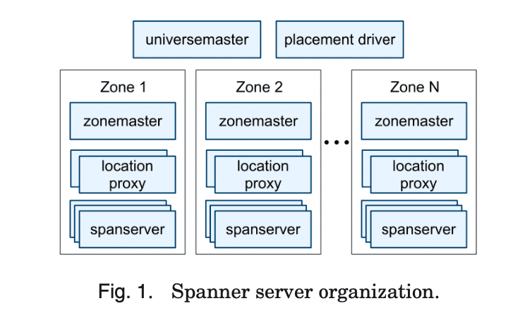
2. One Spanner deployment is called a universe. (Think of a universe as one Spanner cluster.)

3. A Spanner cluster is managed by a set of zones; a zone is an analog grouping of Spanner servers. (Very similar to OB.)

4. The manageable deployment unit is a zone. You can add a zone (add a new datacenter) or remove a zone (turn off some machines). Zones are physically isolated; a datacenter may contain one or more zones, and different groups of machines in a datacenter can form different zones, with data then partitioned across the different zones.

   

5. A zone has one zonemaster and thousands of spanservers. The zonemaster is responsible for assigning data to spanservers.

6. The spanserver responds to client requests.

7. Each zone has a set of location proxies responsible for routing.

8. The universe master and placement driver are currently single points.

9. The universe master displays the status information of all zones.

10. The placement driver communicates periodically with the spanservers to determine which data needs to be relocated (to satisfy load balancing or to upgrade replica constraints); the granularity of relocation is on the order of minutes.

Software Stack

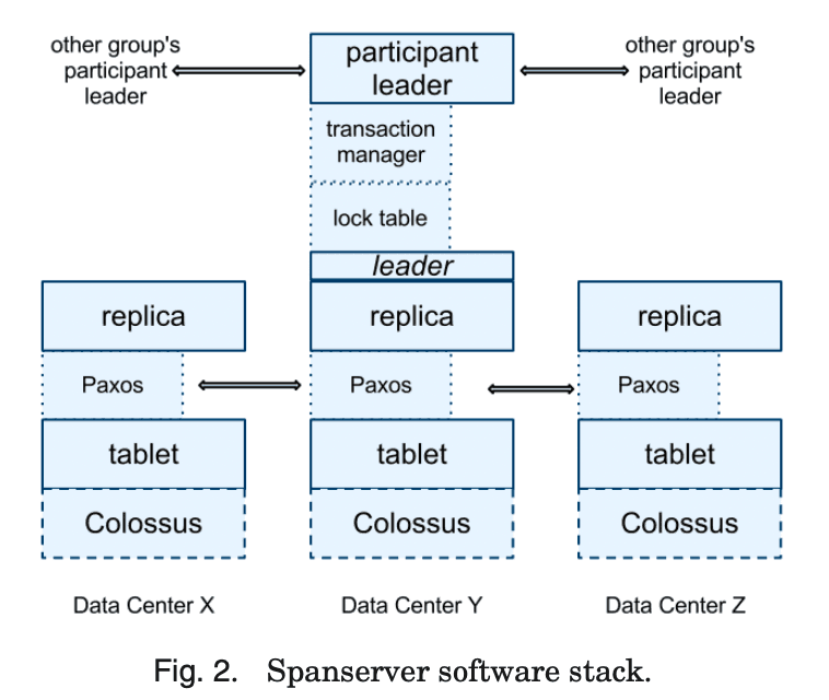
1. At the bottom layer, each spanserver is responsible for 100 to 1000 tablet instances.
2. The tablet is similar to the Bigtable tablet abstraction. It can be understood as a batch of mappings like the following:
   3. (key:string, timestamp:int64) –> string
3. Tablets are organized in B-tree-like files and a WAL log.
4. All data is stored in Colossus, this distributed file system (the successor to GFS).
5. Each tablet has one Paxos group (in the earliest design, one tablet had multiple Paxos groups).
6. Each Paxos state machine stores its metadata and log in its tablet.
7. Paxos supports a long-lived leader, with the leader based on a time-based leader lease, which defaults to 10s.
8. Each log is actually written twice: once in the tablet’s log, and once in the Paxos log. (This is a current stopgap and will be fully fixed later.)
9. Paxos is pipeline-based, which improves throughput. The pipeline is based on Lamport’s “multi-decree parliament.” Pipelining amortizes the cost of leader election and allows parallel voting across different decrees. Although decrees may be allowed out of order, the implementation still keeps decrees ordered.
10. Paxos implements a consistent, replicated mapping (the data mapping method described earlier); each replica’s key-value mapping is stored in its corresponding tablet.
11. The leader initiates Paxos protocol writes. If a replica is already up to date, it can read the state of the replica’s underlying tablet directly.
12. The leader of each Paxos group implements a lock table for concurrency control (the leader’s long life is the key means of keeping the lock table efficient). The lock table involves two-phase locking.
    14. It maps key ranges to lock states.
    15. When there is a conflict, under optimized concurrency control, long transactions execute slowly.
    16. Operations that require synchronization, such as transactional reads, need to acquire a lock from the lock table; other operations bypass the lock table.
    17. The state of the lock table is volatile.
13. The leader of each Paxos group implements a transaction manager to support distributed transactions.
    11. The transaction manager is used to implement the participant leader; the others are participant slaves.
    12. If a transaction involves only one Paxos group, it bypasses the transaction manager, and the lock table and Paxos can provide the transaction capability.
    13. If a transaction involves multiple Paxos groups, the leaders of the Paxos groups perform two-phase commit. One of the leaders is elected as the coordinator, and the other members of that Paxos group are coordinator slaves.
    14. Each transaction manager’s state is also stored using the Paxos group.
14. The smallest unit for data relocation, replication, and data locality is the directory (a better name would be bucket).
    12. A directory is a contiguous range of keys that share a common prefix.
    13. The application can control the locality of this batch of data by carefully choosing keys.
    14. The data under a directory has the same replica configuration.
    15. A directory can be migrated between different Paxos groups.
    16. Relocation often happens to move data closer to its accessors.
    17. A 50 MB directory can be relocated in just a few seconds.
    18. A Paxos group contains multiple directories.
    19. A Paxos group is not a partition of a single contiguous field-ordered range of the row space.
    20. In fact, a tablet is a container that holds multiple row-space partitions, making it convenient for multiple directories to be accessed together.
    21. If a directory grows very large, it is split into fragments, and the relocation granularity is then done by fragment.
15. movedir is a background task. It can not only relocate a directory within a Paxos group, but also add or remove a directory in one Paxos group to a new Paxos group.
    21. movedir is not a transaction, so as not to block subsequent reads and writes.
    22. It performs data relocation in the background. Once most of the data has been relocated, the remaining data is relocated and its metadata changed via a transaction.
16. Placement can be determined by the application.
    24. The placement language is solely responsible for replica configuration management.
    25. It controls two dimensions:
        26. The type and number of replicas
        27. The geographic placement of replicas
    26. Applications can freely control these, for example having a’s data in 3 replicas in Europe and b’s data in 5 replicas in North America.

Data Model

1. The application data model is based on a key-value, hierarchical directory-bucket model. An application creates one or more databases in a universe. Each database can contain countless schematized tables. Tables are similar to those in relational databases, with rows, columns, and versioned values.

2. The data model is not a purely relational model; rows must have names. Each table must have one or more ordered primary keys.

3. As long as a value is defined for some key (even if it’s null), those rows exist. By choosing the range of keys, you can determine which directories the data is placed in, and thus its locality.

   

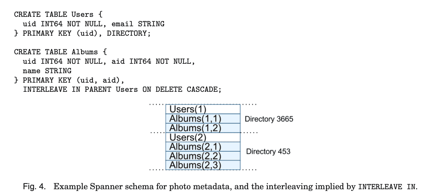
4. The example shows:

   5. Defining table hierarchies through an INTERLEAVE IN declaration in the schema.
   6. The topmost part of a hierarchy is the directory table.
   7. Each row in the directory table has a key, and the rows of its associated subsequent tables related to this key are placed here, arranged in lexicographic order, forming a directory.
   8. ON DELETE CASCADE means that deleting this row of the directory table deletes all related child rows.
   9. This approach preserves the relevance among multiple tables, gives them the same locality, and also yields better performance.

TrueTime

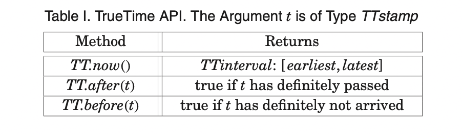
1. The figure above shows the TrueTime API. TrueTime uses TTinterval to represent time, which is an uncertain time interval.
2. The endpoints of a TTinterval are TTstamps.
3. TT.now represents the absolute time of the call. The time epoch is similar to Unix time (it supports leap seconds).
4. The instantaneous error bound is defined as ε, which is half the width of the interval.
5. The average error bound is ε (with an overline).
6. The absolute time of an event is denoted Tabs(e). With tt = TT.now(), we have tt.earliest <= Tabs(Enow) <= tt.latest. Enow is the calling event.
7. GPS and atomic clocks are used as TrueTime references because they have different failure models. The vulnerabilities of GPS reference sources include antenna and receiver failures, local radio interference, correlated failures (e.g., design errors such as incorrect leap-second handling and spoofing), and GPS system outages. Atomic clocks can fail in ways unrelated to GPS and to each other, and over long periods they can drift significantly due to frequency errors.
8. Each datacenter has a time master, and each machine runs a timeslave background process. Most masters have GPS receivers with dedicated antennas; these masters are physically separated to reduce the effects of antenna failures, radio interference, and spoofing. The remaining masters (which we call Armageddon masters) are equipped with atomic clocks. An atomic clock is not that expensive: the cost of an Armageddon master is roughly comparable to that of a GPS master. The time references of all masters are regularly compared against one another. Each master also cross-checks the rate at which its reference time advances against its own local clock, and evicts itself if there is a large divergence. Between synchronizations, an Armageddon master advertises a slowly increasing time uncertainty derived from a conservatively applied worst-case clock drift. The uncertainty advertised by GPS masters is typically close to zero.
9. Each daemon polls a variety of masters to reduce sensitivity to errors from any single master. Some of these are GPS masters chosen from nearby datacenters; the rest are GPS masters from more distant datacenters, along with some Armageddon masters. The daemon applies a variant of Marzullo’s algorithm to detect and reject liars, and synchronizes the local machine’s clock with the non-liars. To protect against a broken local clock, machines that exhibit a frequency deviation greater than the worst-case bound derived from component specifications and the operating environment are evicted. Correctness depends on ensuring that the worst-case bound is enforced.
10. Between synchronizations, the daemon advertises a slowly increasing time uncertainty. ε is derived from conservatively applied worst-case local clock drift. ε also depends on the time master’s uncertainty and the communication delay to the time master. In our production environment, ε is typically a sawtooth function of time, varying from about 1 to 7 ms over each poll interval. As a result, ε is 4 ms most of the time. The daemon’s poll interval is currently 30 seconds, and the currently applied drift rate is set to 200 microseconds per second; together these produce the sawtooth bounds from 0 to 6 ms. The remaining 1 ms comes from the communication delay to the time master. Departures from this sawtooth are possible in the presence of failures. For example, occasional time-master unavailability can cause datacenter-wide increases in ε. Likewise, overloaded machines and network links can cause occasional localized ε spikes. Because Spanner can wait out the uncertainty, variations in ε do not affect correctness, but if ε increases too much, performance may degrade.

Concurrency Control

1. How to implement externally consistent transactions, lock-free snapshot transactions, and non-blocking reads in the past.

   

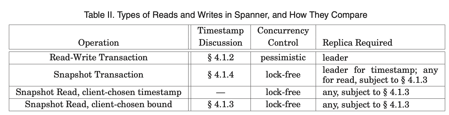
2. A standalone write becomes a read-write transaction, and a snapshot-less standalone read becomes a snapshot read; both retry internally, with no need for the client to retry.

3. Snapshot transactions can enjoy the benefits of snapshot isolation.

   4. A snapshot transaction must declare that it has no write operations. It is not simply a read-write transaction without writes.
   5. A snapshot read executes with an acquired system time and without locking, so subsequent writes are lock-free.
   6. In a snapshot transaction read, any replica that is up to date can serve the read.

4. In a snapshot read transaction, the client can choose a timestamp or provide an upper bound for the desired timestamp range, letting Spanner pick a time.

5. In a snapshot transaction or snapshot read, once a timestamp is chosen, it commits, unless the data at that timestamp has been GC’d. The client can avoid constant retries.

   9. When a server fails, the client uses the timestamp and current read position to read from another server.

6. Paxos leader lease

   10. The leader lease is about 10s. When a candidate leader obtains a majority, it acquires the leader lease.
   11. When the leader lease is about to expire, the current leader initiates a vote, and replicas carry a lease vote in a successful write response.
   12. The leaders of each Paxos group are disjoint.
   13. A leader can step down to a slave by means of a lease vote.

7. Read-write transactions use strict two-phase locking.

   15. After acquiring all locks and before releasing any, they are assigned a timestamp; this timestamp is the timestamp of the Paxos write that represents the transaction’s commit.
   16. Monotonicity
       17. Paxos writes remain monotonically increasing, even across leaders. By exploiting the disjointness of leaders, monotonic increase across leaders is enforced.
       18. A leader can only assign timestamps within its own term.
       19. Whenever a timestamp is assigned, Smax is advanced to s to ensure disjointness.

8. Enforcing external consistency

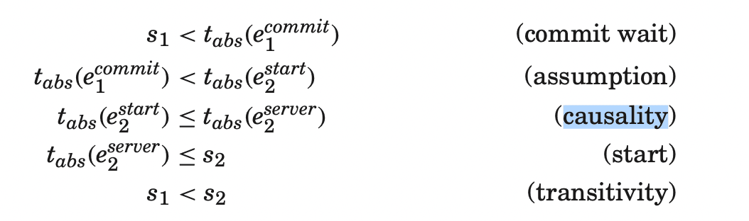
   21. If T2’s start time is after T1’s commit time, then T2’s commit time must be greater than T1’s commit time.

   22. Use E-i-start and E-i-commit for the start event and commit event of a transaction Ti (a mathematical expression, hard to write in Markdown, so escaped here), and denote Ti’s commit timestamp by Si.

   23. The time at which write transaction Ti’s commit arrives at the coordinator leader is E-i-server.

   24. Ti’s commit timestamp Si is no less than TT.now().latest. The participating leader is irrelevant.

   25. Commit wait. The coordinator ensures that clients cannot see Ti’s committed data until TT.after(si) is true. Commit wait ensures that si is less than Ti’s absolute commit time.

       

   26. Each replica’s synchronization time is called the safe time, Tsafe = min(T-safe-paxos, T-safe-TM).

       27. Each Paxos state has a safe time T-safe-paxos, and each transaction manager has a T-safe-TM.
       28. T-safe-paxos is simple: it is the time of the highest applied Paxos write. Paxos writes are monotonically increasing and ordered.
       29. T-safe-TM is more complex.
           30. When there are no prepared transactions, it is infinite. That is, the transaction is in the two-phase commit period.
           31. During two-phase commit, each participant knows the lower bound of a prepared transaction’s timestamp.
           32. Let S-i/g-prepare denote the prepare timestamp of the prepare record, and guarantee that the transaction’s commit time si >= S-i/g-prepare.
           33. T-safe-TM = min(over all transactions)(S-i/g-prepare) - 1 in time.

9. A snapshot transaction performs two-phase commit.

   35. It assigns a timestamp S-read and then reads with S-read.
   36. The simplest approach: when a transaction starts, S-read = TT.now().latest. But sometimes problems arise.
   37. When a replica’s T-safe is not yet sufficient, it blocks on S-read.
   38. To reduce blocking, Spanner chooses the maximum time that preserves external consistency.

10. Read-write transactions

    40. Reads in a read-write transaction use the wound-wait method to avoid read-write locks.
    41. The request is sent to the leader to request read locks and read the latest data.
    42. If the client transaction is reopened, it uses keepalive to avoid the participant leader timing out.
    43. The client chooses the coordinator Paxos group, then sends a commit message with the coordinator id and the buffered write operations to all participant leaders.
    44. When a non-coordinator leader first requests a write lock, it chooses a prepare timestamp larger than any prior transaction’s timestamp, logs the prepare record via Paxos, and notifies the coordinator leader of its prepare timestamp.
    45. When the coordinator first requests a write lock, it skips the prepare phase. After receiving responses from all participant leaders, it chooses a timestamp as the timestamp of the entire transaction (which should be the commit timestamp).
        46. The commit timestamp s is greater than or equal to all prepare timestamps. In fact, it is greater than TT.now().latest at the moment the coordinator receives the commit message. It is also greater than all timestamps of all prior transactions.
        47. The coordinator then logs this commit record via the Paxos log.
    46. Only a Paxos leader can request locks. The lock state is logged only during the transaction’s prepare phase.
        49. If a lock is lost before prepare (due to deadlock, a Paxos leader change, timeout, etc.), the participant gives up.
        50. Spanner guarantees that it only logs a prepare or commit record when all locks are held.
        51. If the leader changes, the new leader restores the lock state of all prepared-but-not-yet-committed transactions before accepting new transactions.
    47. Before all of the coordinator’s replicas apply the commit record, the coordinator’s leader waits until TT.after(s), so that it can obey the commit-wait rule, because it must ensure TT.now().latest has indeed become the past. Typically this wait is twice the average bound ε. This wait can run in parallel with Paxos communication.
    48. After commit-wait, the coordinator sends the commit timestamp to the client and to all participant leaders.
    49. Each participant logs the transaction’s output via the Paxos protocol, then applies this timestamp, and finally releases the locks.

11. Snapshot transactions.

    56. Before assigning a timestamp, this read requires negotiation among all involved Paxos group leaders.
    57. Spanner then requires a scope expression, which summarizes the keys of this read transaction and then triggers the independent query.
    58. If this scope’s values involve only one Paxos group, the client sends this snapshot transaction directly to that Paxos leader.
        59. That leader assigns an S-read and executes the read.
        60. For single-node reads, Spanner can do better than TT.now().latest.
        61. Define LastTS() as the timestamp of the last committed write transaction.
        62. If there are no prepared transactions, simply set S-read = LastTS() to satisfy external consistency.
    59. If multiple Paxos groups are involved:
        53. The complex approach: all participant leaders need to negotiate S-read together based on each LastTS().
        54. The simple approach (the current one): the client does not perform a round of negotiation and directly chooses a safe S-read = TT.now().latest.
    60. Schema-Change transactions:
        56. TrueTime supports atomic schema changes.
        57. Using a standard transaction is infeasible because the participants number in the millions.
        58. Bigtable supports atomic schema changes within a single datacenter, but this operation blocks all operations.
        59. The current schema-change transaction is a lock-free variant of a standard transaction.
        60. The first step assigns a future timestamp during the prepare phase, to reduce the impact on the current workloads of thousands of servers.
        61. Read and write requests that obviously depend on this schema synchronize against the timestamp t registered for the schema change.